Matplotlib’s State-Machine Approach

Matplotlib’s matplotlib.pyplot module is designed to feel like MATLAB. Rather than explicitly creating figure objects, the pyplot module maintains state as soon as it is imported. If you come from a more object-oriented background, this may seem like a bit of magic. It can be a bit difficult to know what Matplotlib is doing for you in the background, but it does allow you to get up and running with fewer lines of code.

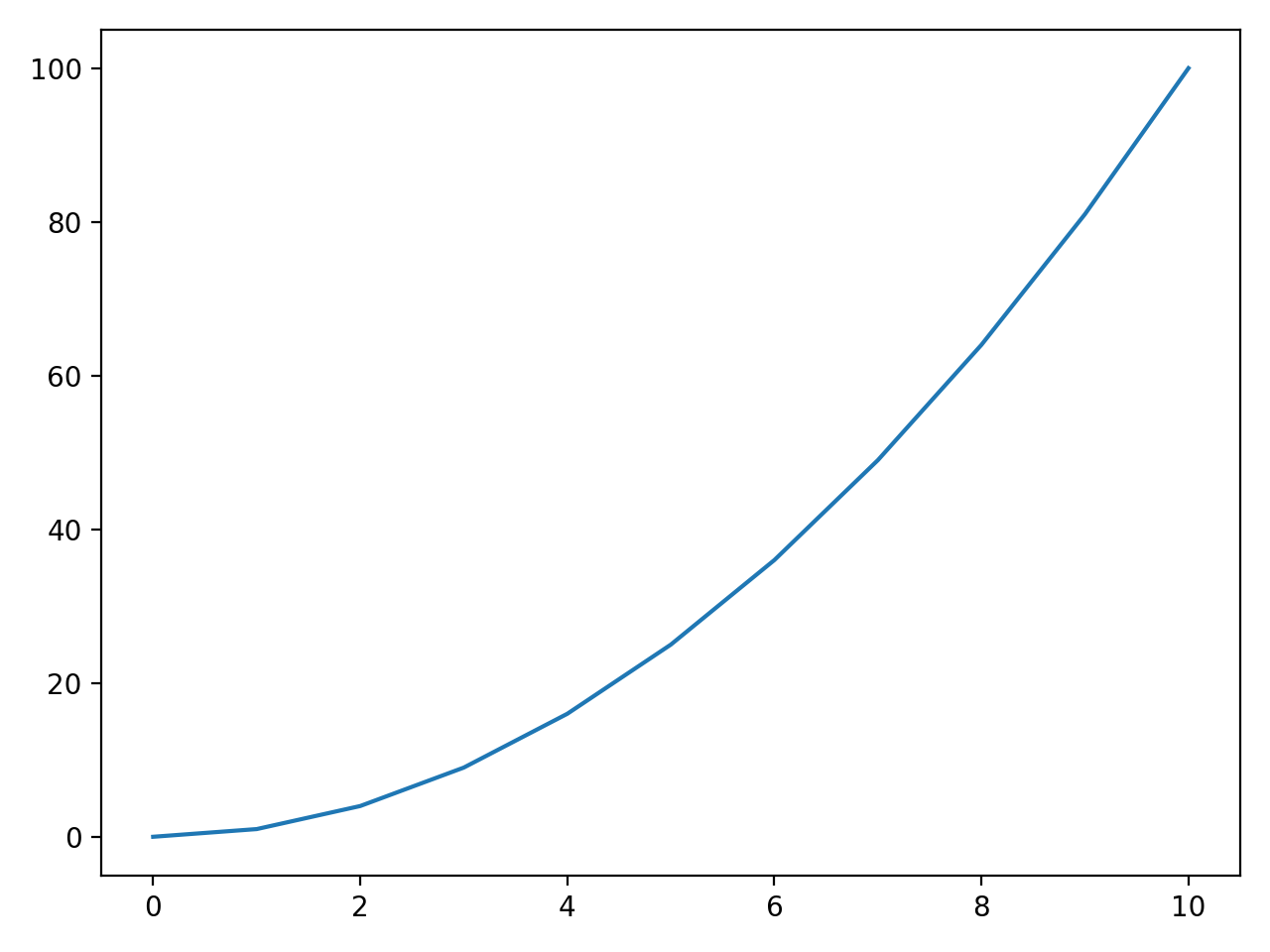
Let’s take a look of a simple example, plotting a single curve:

import matplotlib.pyplot as plt # immediately plt is keeping track of state

# first 10 squares
squares = [x**2 for x in range(11)]

plt.plot(squares)
plt.show()

This is about as simple as a Matplotlib figure can get. Given x, a Python list of the first 10 squares, Matplotlib gives us a line plot. The pyplot module is inferring a lot here. Notice that we did not specify our x and y axes. We didn’t even tell it Matplotlib that we were looking to plot a curve here!

Also note that we never instantiated an object from the pyplot module. Instead, we are calling the module directly. First, we feed our data into plt.plt(x), then we call plt.show() to render our figure. If we were to call plt.show() again without passing the data back into plt.plot(), Matplotlib will not render the figure a second time. That is because Matploglib clears the state of our plot as soon as we call show`.

Adding some Details

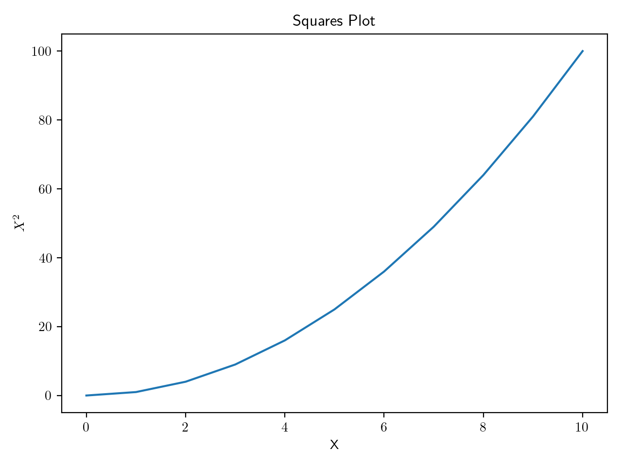
While pyplot can infer a lot of the details for us, we will need to handle axis labels and titles ourselves.

plt.plot(squares)
plt.title('Squares Plot')
plt.ylabel(r'$X^{2}$')
plt.xlabel('X')
plt.show()